Multi-Depot Routing Problem with Van-Based Driverless Vehicles: A Heuristic Approach

Introduction

Urbanization, population growth, the rise of e-commerce, and new technologies have dramatically changed how goods are delivered in urban areas. To make these deliveries more efficient, better coordination is needed between different delivery participants and transportation methods. This paper introduces the multi-depot routing problem with van-based driverless vehicles (MDRP-VBDV), which builds upon the multi-depot routing problem (MDRP) and uses a “mothership” concept where vans carry driverless vehicles.

Van-based driverless vehicle.

As e-commerce and home delivery services expand, logistics companies are constantly seeking more cost-effective delivery solutions. Collaboration between multiple depots can help achieve these goals. Generally, MDRP involves optimizing the routes of a fleet of vehicles originating from multiple depots to serve customers, minimizing costs such as distance. The way depots work together can vary, which leads to different MDRP characteristics. For example, a vehicle might return to its original depot or any depot after making deliveries. For MDRP where vans can depart from one depot and return to another, the number of vans in each depot may change, and some depots might have no vans. To ensure the delivery system is sustainable, the number of vans at each depot should stay the same at the start and end of deliveries.

Background

Increasing labor costs, driven by aging populations and economic growth, further complicate delivery logistics. Moreover, the growth of cities has led to rising traffic congestion, pollution, and noise. To address these issues, there’s been significant development of new technologies and concepts for delivering goods. This paper explores the use of driverless vehicle technology for goods delivery. Jennings and Figliozzi have provided detailed summaries on the subject. Driverless vehicle delivery is expected to lead to fewer accidents and lower carbon emissions. Some logistics companies, such as JD.com and Meituan, have already tested driverless vehicles. Public willingness to use driverless vehicles has also been studied. At this stage, driverless vehicles face technical and policy limitations that make independent delivery difficult. The “mothership” concept improves the practicality of driverless vehicle delivery by utilizing vans to carry and deploy driverless vehicles.

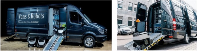
Mercedes-Benz Vans and Starship Technologies, for example, have teamed up to develop van-based delivery robots, with Starship Technologies providing autonomous robots for last-mile deliveries. Workhorse has also launched city delivery services that use a combination of trucks and drones, while Amazon is testing airships with small drones for last-mile delivery. Boysen et al. and Yu et al. have also studied van-based driverless vehicle delivery (VBDVD) in urban environments.

VBDVD offers significant advantages:

1. Efficiency: Driverless vehicles are often slow for safety reasons and alone may cause traffic problems. VBDVD solves this.
2. Reduced Costs and Pollution: VBDVD can significantly reduce costs for logistics companies by decreasing labor costs. Driverless vehicles can reduce urban pollution because they are battery-powered.
3. Flexibility: Vans act as mobile depots. They drop off driverless vehicles and can recover broken-down driverless vehicles. The scheduling plans are more flexible.
4. Practicability and Safety: VBDVD is more practical and safer than van-based drones in urban environments. Drones are more sensitive to bad weather and create dangerous environments for delivery.

Research Focus

While VBDVD has been explored, better coordination between vans and driverless vehicles in the mothership concept is still needed. This paper considers a system where vans, each carrying several driverless vehicles and goods, depart from a depot, visit stops within urban regions, and release the driverless vehicles. These driverless vehicles then deliver goods to customers and return to the nearest stop or depot after completing their deliveries. Driverless vehicles that return to stops can then be picked up by any available van. After all deliveries, all vans and driverless vehicles return to their depots. The number of vans at each depot remains constant before and after delivery, but the driverless vehicles in each depot can be changed or moved to increase distribution.

This research contributes in the following ways:

• Introduces the multi-depot routing problem with van-based driverless vehicles based on MDRP and VBDVD.
• Proposes multi-depot joint distribution, in which the number of vans in each depot remains unchanged and vans can depart from one depot and return to another, to maintain a sustainable system and advance cooperation of multiple depots.
• Proposes van-van joint distribution where driverless vehicles can be dropped off and picked up by different vans.
• Formulates a mixed-integer programming model and designs a heuristic algorithm to solve the problem.
• Analyzes the impact on scheduling plans of the maximum number of driverless vehicles per van, and of the travel time of the driverless vehicles.

Literature Review

To provide context for the MDRP-VBDV problem, this section reviews relevant existing studies on MDRP and the mothership concept, similar to VBDVD, distinguishing them by their characteristics and applications. It will further examine multi-depot joint distribution and van-van joint distribution.

Multi-Depot Routing Problem (MDRP)

MDRP is an extension of the VRP, with three main types depending on the cooperation level among depots, van ownership, and the sustainability of the distribution system:

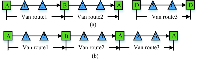
1. Fixed MDRP (F-MDRP): Each vehicle route must start and end at the same depot (see Fig. 2a). A common solution approach is to divide F-MDRP into multiple single-depot routing problems. In early applications, it was popular to have each depot serve customers within a fixed area, but this approach lacks flexibility.

   

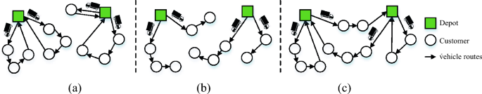
   Three types of multi-depot routing problems.

2. Multi-Depot Open Routing Problem (MDORP): Each vehicle starts from one depot and does not need to return (Fig. 2b). This is seen frequently in practice, especially when companies do not have their fleet or their vehicles can’t meet the delivery needs. MDORP appears in other transportation problems.

3. Multi-Depot Joint Distribution: Vehicle routes can start and end at different depots (Fig. 2c). The lowest delivery cost may not involve routes around only one depot, and the routes between two different depots may lead to the lowest cost. To maintain the sustainability of the delivery system, the number of vans at each depot should remain unchanged.

The Mothership Concept

The concept of applying the mothership emerged first in military and environmental monitoring, and then it has been applied to delivering goods. There are two main delivery methods on the mothership concept:

1. Van-based drone delivery (VBDD).
2. Van-based driverless vehicle delivery (VBDVD).

Compared with drones, driverless vehicles have better loading capacity, longer duration, and safer operation conditions. VBDVD can be divided into two cases, depending on whether the stops where vans drop off or pick up drones/driverless vehicles are:

1. Customer locations.
2. Special locations.

These cases are explained in more detail in Fig. 3.

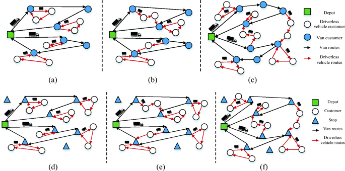
Six deliveries on the mothership concept.

Different driverless vehicle/drone routes are:

1. The starting and ending stops are the same.
2. The starting and ending stops are different (vans move to other stops for recovering driverless vehicles/drones).
3. The ending stop and the starting stop are in two different van routes (van-van joint distribution).

Summary of Relevant Studies

Some studies related to the mothership concept are summarized in Table 1.

Table 1: Some studies related to the mothership concept.

[Table 1 details the information from the original document and is replaced with the text for brevity]

Problem Description and Model

Problem Statement

The MDRP-VBDV problem has several key characteristics:

• Multiple depots where a homogeneous fleet of vans and driverless vehicles is available.

• Vans cannot directly deliver goods because of traffic congestion.

• Driverless vehicles can deliver goods.

• There are six types of driverless vehicle routes, shown in Fig. 4.

  

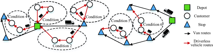
  Six types of driverless vehicle routes.

• Each van has spaces for driverless vehicles and goods, and each van is paired with a fixed number of driverless vehicles.

• Driverless vehicles are dropped off at the stop and return to it at the end of delivery. These driverless vehicles are loaded with goods for the next delivery, and lastly, vans depart for the next depot/stop.

The operations are outlined in Fig. 5.

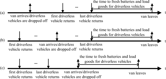
Three cases for operations at stops along time.

Mixed Integer Programming Model

The objective is to minimize the delivery cost, which includes fixed and transportation cost.

The notations for this model are defined as follows:

Table 2: Notations

[Table 2 details the information from the original document and is replaced with the text for brevity]

The objective function minimizes the delivery cost (1), which contains the fixed cost of vans and the transportation cost of vans and driverless vehicles:

$${text{min}}left( {sumlimits{k in K} {sumlimits{{i in V{0} }} {sumlimits{{j in V{1} }} {c{1} x{kij} } } } + sumlimits{k in K} {sumlimits{{i in V{0} cup V{1} }} {sumlimits{{j in V{0} cup V{1} }} {c{2} x{kij} l{ij} } } } + sumlimits{r in R} {sumlimits{i in V} {sumlimits{j in V} {c{3} x{rij} l_{ij} } } } } right).$$ (1)

The constraints for the model are as follows:

1. Assures the number of vans at each depot remains unchanged (2).
2. Each van is dispatched no more than once (3).
3. The number of vans arriving at one stop is equal to that departing from the stop (4).
4. One stop can be visited by vans only once (5).
5. All dispatched driverless vehicles return to the depots after the delivery (6).
6. The number of driverless vehicles arriving at one stop equals the number departing (7).
7. The number of driverless vehicles arriving at one customer is equal to the number departing from the customer (8).
8. One customer can be visited by only one driverless vehicle (9).
9. Each driverless vehicle is dispatched from one stop no more than once (10).
10. Time of vans cannot exceed the maximum travelling time (11).
11. Time-related constraints for driverless vehicles (12) and (13).
12. Time-related constraints for vans (14)-(16).
13. Constraint of driverless vehicles (17).
14. Capacity constraints for the vans (18) and (19).
15. Capacity constraints for the driverless vehicles (20) and (21).
16. Constraints on the variables (variable definitions 22-24).

Methodology

The problem is complex, especially with multi-depot and van-van joint distribution, which has an effect on solving MDRP-VBDV. An iterated heuristic algorithm is designed to solve MDRP-VBDV to balance the quality and speed of solving the problem.

Construct Primary Solutions

The general structure to construct the primary solutions is shown in Algorithm 1.

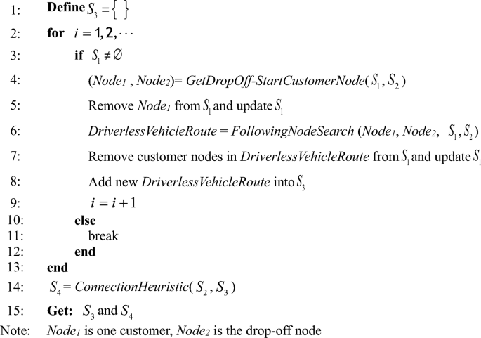
Algorithm 1: ConstructPrimarySolutions (S1, S2).

The procedure constructs the primary solutions by creating driverless vehicle routes (lines 1-13) and constructing van routes (line 14). The procedure GetDropOff-StartCustomerNode is used to select the drop-off node (depot/stop) and the first customer node in one complete driverless vehicle route. Two strategies are used.

1. Select the drop-off node and the first customer node with the shortest distance.

2. Algorithm 2.

   

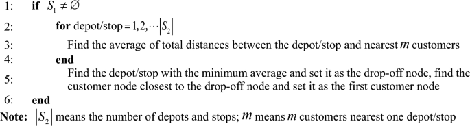
Algorithm 2: GetDropOff-StartCustomerNode (S1, S2).

After getting the drop-off node and the first customer node, we apply FollowingNodeSearch to select the following customers and the pick-up node sequentially for constructing complete driverless vehicle routes. The nearest distance strategy and the random selection strategy are used in FollowingNodeSearch. Ensure the chosen nodes subject to all constraints. The constraints involve the time window of depots, the maximum capacity for goods and the maximum travelling time of driverless vehicles. The procedure FollowingNodeSearch is repeated until no customer node is left, finally, select the nearest stop or depot as the pick-up node to make a complete driverless vehicle route.

To construct complete van routes, we designed the procedure ConnectionHeuristic. The general structure of the procedure is sketched out in Algorithm 3.

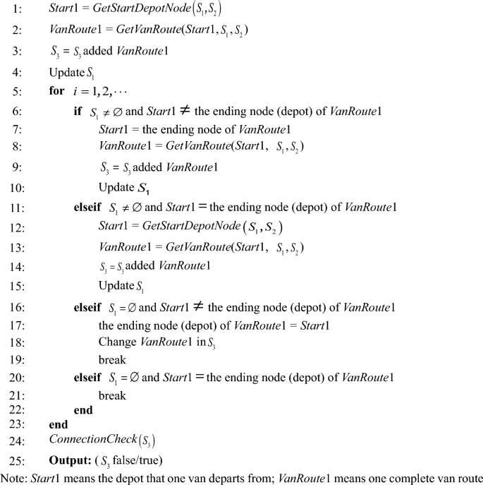
Algorithm 3: ConnectionHeuristic (S1, S2).

The procedure GetStartDepotNode in Algorithm 3 is applied to choose one depot as the starting node of one van route. GetStartDepotNode is based on the nearest distance criterion. After ensuring the starting node of one van route, GetVanRoute is run to get one complete van route. Two strategies are used in GetVanRoute, one is the nearest distance criterion, and another is the shortest traveling time criterion, which thus yields a significant difference in initial solutions. Each van route should meet the constraints involving the maximum capacity of vans for goods, the maximum number of driverless vehicles in one van and the maximum traveling time of vans.

The procedure GetVanRoute is shown as follows.

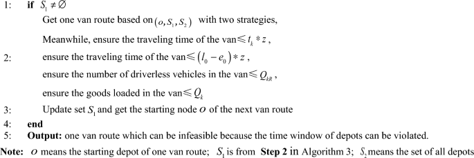
Algorithm 4: GetVanRoute (o, S1, S2).

In Algorithm 3, lines 6–22 keep the number of vans at each depot unchanged. Lines 11–15 lead to unconnected loops rather than connected loops only, which increases solution diversity. The procedure ConnectionCheck is aimed at judging whether the scheduling plans meet the time window of depots by introducing variable w{i}, w{i} is the waiting time of one van at stop i.

The scheduling plans by two methods.

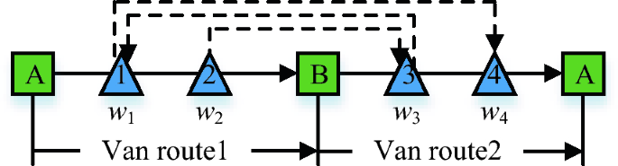
An example to explain ConnectionCheck.

Constraints (25) and (26) ensure that each van travels in the time window of the depots. Constraints (27)–(29) make sure that the time when one van departs from one stop is after the time when all driverless vehicles return to the stop.

Iterated Optimization

This paper uses an iterated neighborhood search approach with destroy and repair operators. The destroy and repair operators reduce the number of vans. The neighborhood search operators reduce the delivery cost.

The structure of the heuristic algorithm is depicted in Fig. 8.

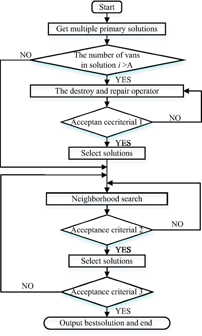
Heuristic flowchart.

To avoid local optimization, this algorithm starts with multiple primary solutions. Acceptance criteria 1, 2 and 3 are the maximum iterated numbers in relative loops. The main steps are as follows:

1. Select solutions where more vans are used than a set parameter (A), and then improve them with destroy and repair operators. Let the improved solutions go to step 2.
2. Improve the solutions from step 1 by the neighborhood search operators and reserve the better solutions until meeting acceptance criteria 3.

Destroy and Repair

The destroy and repair operators include the insert operator in condition② and the PD operators in “Neighborhood search”.

Neighborhood search

The neighborhood search approach is to reduce the cost. It uses the insertion and swap operators with other specialized methods like insert and swap operators for different scenes, changing only the pick-up nodes (conditions⑤), changing only drop-off nodes (conditions⑥), and by changing simultaneously drop-off nodes and pick-up nodes (PD operators). The operators to change starting depots and ending depots of van routes (SE operators) are applied.

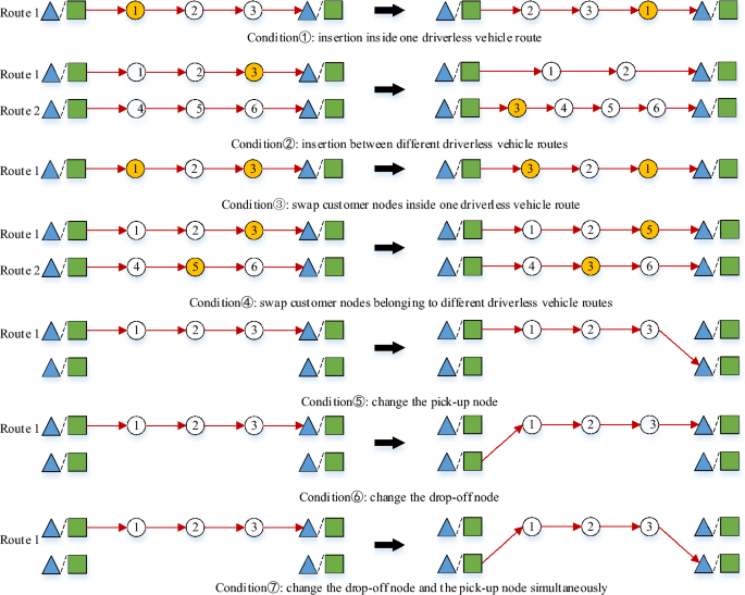
Insert, swap and PD operators.

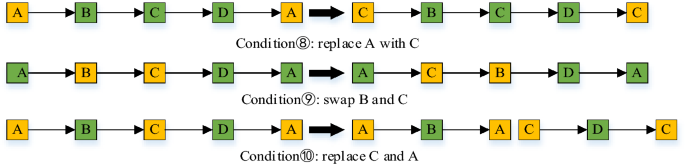
SE operators.

SE operators include three classes (replace, swap and 2-replace).

Computational Study

To assess the performance of the heuristic algorithm, the authors generated 27 instance types with different depot, stop, and customer node counts. Then, the effectiveness of the heuristic algorithm is analyzed concerning the number of driverless vehicles per van and maximum travel time of driverless vehicles.

Instance Generation

The locations of depots and stops are generated, and the serving time of customers is:

• Category A (CGA): (t{si} in left( {0,,0.05t{r} } right)), (d{i} in left( {0,,0.25Q{r} } right))
• Category B (CGB): (t{si} in left( {0.05t{r} ,,0.1t{r} } right)) and (d{i} in left( {0,,0.25Q_{r} } right))
• Category C (CGC): (t{si} in left( {0,,0.1t{r} } right)) and (d{i} in left( {0,,0.25Q{r} } right))
• Category D (CGD): (t{si} in left( {0,,0.05t{r} } right)) and (d{i} in left( {0.25Q{r} ,,0.5Q_{r} } right))
• Category E (CGE): (t{si} in left( {0.05t{r} ,,0.1t{r} } right)) and (d{i} in left( {0.25Q{r} ,,0.5Q{r} } right))
• Category F (CGF): (t{si} in left( {0,,0.1t{r} } right)) and (d{i} in left( {0.25Q{r} ,,0.5Q_{r} } right))
• Category G (CGG): (t{si} in left( {0,,0.05t{r} } right)) and (d{i} in left( {0,,0.5Q{r} } right))
• Category H (CGH): (t{si} in left( {0.05t{r} ,,0.1t{r} } right)) and (d{i} in left( {0,,0.5Q_{r} } right))
• Category I (CGI): (t{si} in left( {0,,0.1t{r} } right)) and (d{i} in left( {0,,0.5Q{r} } right))

Parameters are shown in Table 3.

Table 3: The parameters

[Table 3 details the information from the original document and is replaced with the text for brevity]

Instances

To improve the speed of solving instances, different population sizes and iterations are set for different instances. In this paper, the population size is 200 and the iterations are 50 for the instances with 15 customers or 30 customers. The population size is 400 and the iterations are 300 for the instances with 50 customers.

The results are presented in Table 4.

Table 4: The solutions for instances.

[Table 4 details the information from the original document and is replaced with the text for brevity]

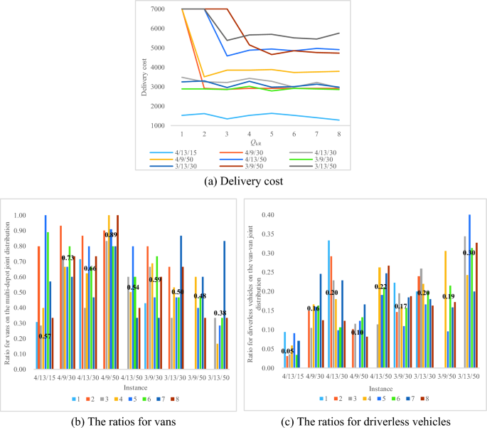
As depicted in Fig. 11, the ratios in blue are the number of vans dispatched on the multi-depot joint distribution divided by the total number of vans dispatched, the ratios in red are the times of driverless vehicles dispatched on the van-van joint distribution divided by the total times of driverless vehicles dispatched.

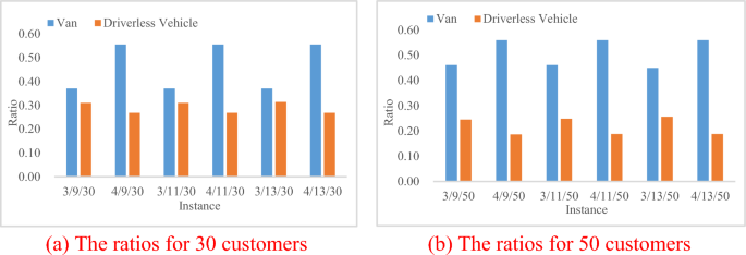
Fig. 11: The ratios for vans and driverless vehicles.

Analysis and Methods

The delivery cost decreases as the number of depots/stops increases.

Analysis of the Heuristic Algorithm

The study compares the performance of this heuristic algorithm with an adaptive genetic algorithm (IGA). Results are shown in Table 5.

Table 5: The solutions of two algorithms.

[Table 5 details the information from the original document and is replaced with the text for brevity]

Table 5 indicates that this designed algorithm is mostly better than IGA. The best and average delivery costs obtained by this designed algorithm are smaller than those by IGA, which indicates that this designed algorithm can solve instances in-depth. For most instances, a value representing deviation between the average and best delivery costs obtained by this designed algorithm is smaller than those by IGA, which indicates that this algorithm can steadily solve instances.

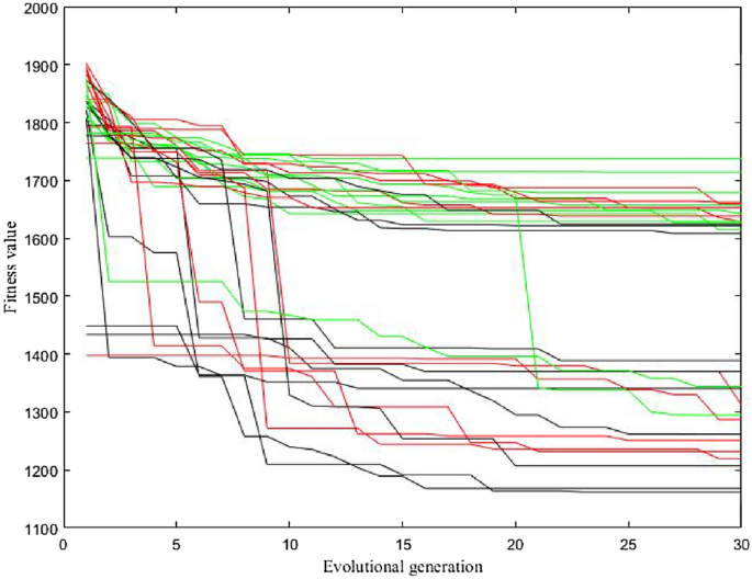
The convergence processes under different strategies.

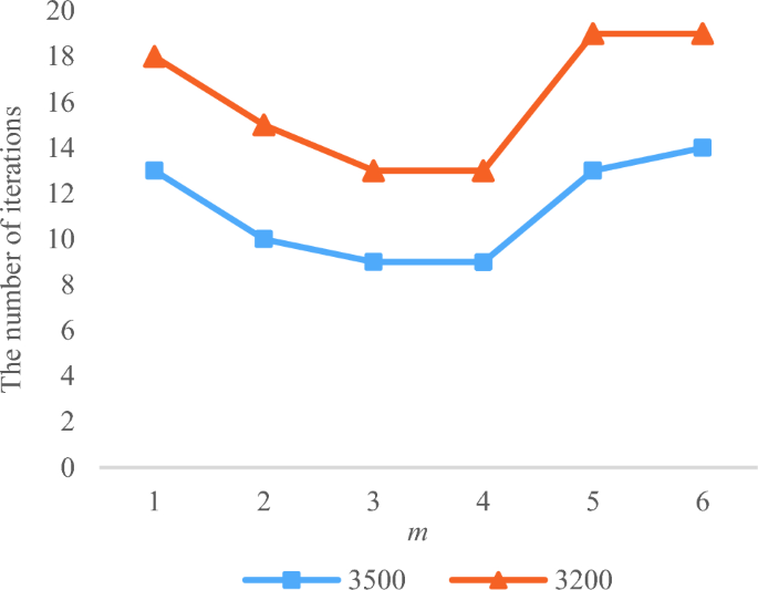
The number of iterations under different m.

Sensitivity Analysis

Sensitivity analyses explored the influence of (Q{kR}) (the maximum number of driverless vehicles per van) and (t{r}) (the maximum traveling time of driverless vehicles).

Table 6: The delivery plans under different (Q_{kR}).

[Table 6 details the information from the original document and is replaced with the text for brevity]

The delivery cost firstly decreases and later remains unchanged as (Q_{kR}) increases (Fig. 14a).

Delivery cost and the ratios for vans or driverless vehicles under different (Q_{kR}).

Table 7: The delivery plans under different (t_{r}).

[Table 7 details the information from the original document and is replaced with the text for brevity]

The delivery cost decreases when (t{r}) varies from 30 to 60 and remains unchanged when (t{r}) varies from 60 to 70 (Fig. 15a).

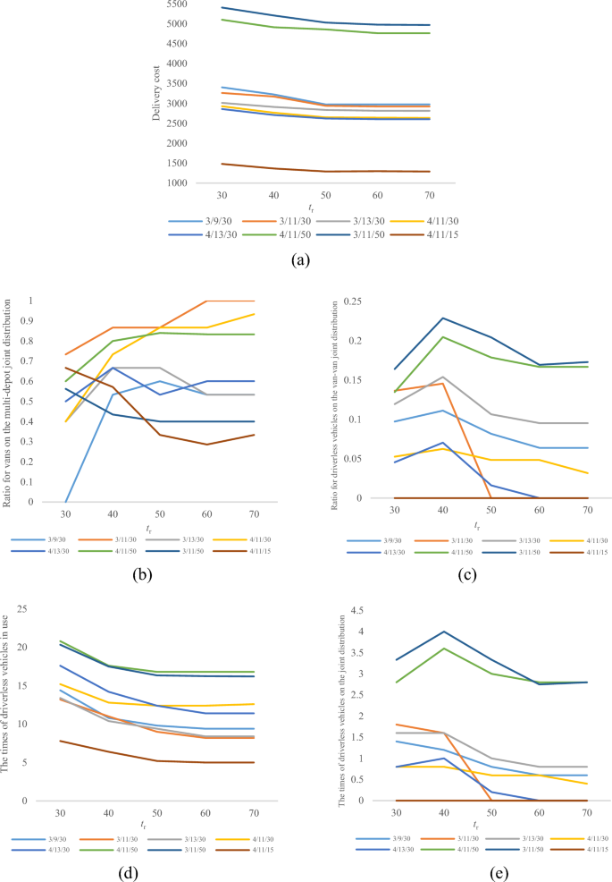
*Delivery costs, the ratios and the times of driverless vehicles under different t_{r